An Introduction to Data Structures in JavaScript
22 August 2018
Hello everyone. Back again after another long hiatus. I have been buried in trying to find a job this summer. It has been a long and intense road so far, but I have already learned a lot in my post boot camp life. One of the things I have been learning are the computer science fundamentals many larger companies require you to know to be successful in their technical interviews. I interviewed at the beginning of August. It was very intense, and while I was ultimately rejected, I found all of the time I devoted to learning data structures and algorithms to be incredibly valuable. Anyone who has graduated from a boot camp should take the time to learn the concepts I am going to discuss in my next several posts. Even if an opportunity does not require you to know these concepts to interview with them, if you ever want to interview at a larger tech company like Google, Microsoft, or Facebook, you are going to need to be familiar with the many type of data structures and sorting algorithms found across the computing world.
Today I am going to give a basic overview of the most common data structures that anyone working in programming should know. In the future, I will try to write some posts delving into implementing these in JavaScript. A lot of the most common resources out there for this topic are in languages like Python, Java, or even C++ so I thought it would be valuable to go over these concepts for web developers that may not be familiar with those languages.
To begin, a list of all of the basic data structures that may appear on a coding interview are in no particular order:
- tree
- heap
- trie
- linked list
- graph
- hash table
- queue
- stack
Before I dive into a brief description of each, concepts you must have a basic understanding of is Big-O time and space complexities. An excellent overview of these concepts can be found in the book Cracking the Coding Interview. The book is also floating around for free illegally on-line, but I won’t link to a place to download here. An reference for Big-O is the Big-O Cheat Sheet.
Trees - Binary Search Trees, Heaps, and Tries
From Wikipedia:
A tree data structure can be defined recursively (locally) as a collection of nodes (starting at a root node), where each node is a data structure consisting of a value, together with a list of references to nodes (the “children”), with the constraints that no reference is duplicated, and none points to the root.
Trees are useful because they offer faster search, insertion, and deletion then other common ordered data structures, like arrays. The average time complexity to search, insert, or deletion from an unsorted array is O(n), because each action is a function of the size of the array. In the case of a tree, search, insertion, and deletion time complexities are O(log(n)). To understand why this is, lets take a look at one of the most common types of trees: the binary search tree.
Binary Search Trees
A binary search tree is a tree where it’s nodes are sorted so that, starting from the root node, items on the left side of the tree are less than the root and items on the right side of the tree are greater than the root. This holds true for each subsequent level of the tree, with each node having a left child less than itself and a right child greater than itself.
The reason binary search trees are more efficient at search, insertion, and deletion than an unsorted array is that as each level is traversed a question is asked: would the node we are looking for be found in the left or the right subtree? Each time this question is answered, a new level is entered and half of the remaining nodes to be searched are removed. This continuous halving of the set to be searched can be represented by the logarithmic scale. This is how we arrive at the fact that the time complexity of search, insertion, and deletion for trees is O(log(n)).
For example:

If we are searching for the node 7, the traversal of the tree is as follows:
- Starting at the root, 8: 7 is less than 8, so continue down the left subtree to 3
- At 3: 7 is greater than 3, so continue down the right subtree to 6
- At 6: 7 is greater than 6, so continue down the right subtree to 7
- 7 is our value, so return node
Heaps
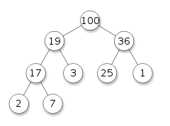
Heaps are also a tree based data structure that has one primary attribute: they satisfy the heap property.
From Wikipedia:
if P is a parent node of C, then the key (the value) of P is either greater than or equal to (in a max heap) or less than or equal to (in a min heap) the key of C. The node at the “top” of the heap (with no parents) is called the root node.
Heaps are also known as priority queues. They have similar strengths to binary search trees in that insert and delete are O(log(n)) time complexity. The primary differences between heaps and binary search trees are the fact that the root node contains the minimum or maximum value based on the structure of the tree and that they are only partially sorted. In this case, heaps are useful if access to the minimum or maximum value is required without a fully sorted dataset. Since the min or max is always accessible, the time complexity accessing these nodes is constant at O(1).
For example, this is a max heap:
Tries
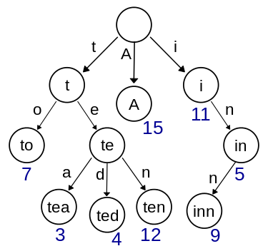
A trie is anther tree type data structure. Nodes in a trie usually store strings. The primary difference between tries and other types of tries is that the position in the trie defines what value is stored in the node, where in other types of trees node values are not limited by position. One of the most common uses for a trie is to store all the words in a language, with the higher levels of the trie containing the shortest words and the lowest level of the trie containing the largest words.
For example, this is small subsection of an English language trie:
Graphs
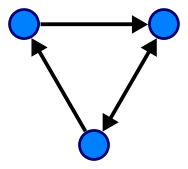
In computer science, graphs are a programmatic implementation of mathematical graphs, where points on displayed on a plain, usually using x and y coordinates. The graph consists of vertex nodes connected by edges. Graphs can be directed, where the edges have a direction associated with them, or undirected where the direction of travel between points is unrestricted. Edges can also have their own value, usually representing distance. In this case, the graph will be considered weighted.
In programmatic terms, graphs are usually represented two ways:
- Adjacency List - A hash map, or basic JS object, that contains each vertex as a key and all of the edges associated with that vertex as an array of values.
- Adjacency Matrix - A multidimensional array where each element is an array. Each array is a row on the matrix, where the indices are keyed to the source vertices. Each index of the top level array is keyed to destination vertices.
For example, this is a directed graph with three vertices connected by three directed edges:
Stack
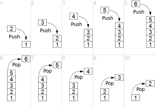
A stack is similar to an array; it is a data structure where orders matters. However, unlike an array a stack abides by the LIFO (last in, first out) principle, where the newest elements are removed first. In terms of an array, this corresponds to the common pop method that removes and returns the last element of an array. Elements are always added to a stack using the push method, adding them to the end of the collection of elements. A common way to visualize a stack is a stack of plates. You can only add new plates to the top of the stack and remove plates from the top as well.
A representation of a stack with push and pop operations:
Queue
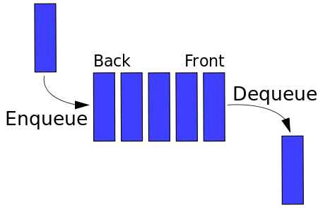
A queue is also like a stack and an array, an ordered data structure. Instead, a queue abides by the FIFO (first in, first out) principle, where the oldest elements are removed first. You man see the common methods associated with queues called enqueue and dequeue. Simply put, enqueue adds to the queue, which corresponds to the push method for arrays. Dequeue removes from the front of the queue, which corresponds to the shift method for arrays. Queues can be conceptualize as people waiting in line where the person waiting in the line longest will be removed first and new persons are added to the back of the line.
That’s it for this post. Next post I will start diving into the actual code in JavaScript that makes up these data structures. I hope this post is helpful for anyone looking to learn computer science fundamentals. I will reiterate it is important to at least be aware that questions based on these data structures exist out there. You may or may not come across these as you try and find a job in the programming world, but I still think it’s valuable to take the time to learn each and every one since you never know when the knowledge may come in handy.